

Introduction
In a recent post, we outlined what a Databricks Lakehouse encompasses and why you may want to utilise one rather than a Data Warehouse and/or Data Lake. Following that introduction, this post will walk through an example use case, including code, for how the Databricks Lakehouse replicates some common warehousing patterns while having the structure and cost of a Data Lake.
Delta Lake Basics
First, it’s worth covering the basics, though feel free to skip ahead to a more real-world example if you are already familiar with Delta Lake.
The heart of the Databricks Lakehouse is Delta Lake, a high-performance file format that has lots of functionality usually only found in Databases and Data Warehouses – schemas, constraints, views, row-level transactions, and more. As such, it also needs to incorporate the basic elements of these components to make it just as useful, such as reading, writing, updating, and deleting data, which are covered below.
Writing to Delta Lake
Writing data to DeltaLake is a simple operation akin to saving an Excel document or creating a new table in SQL. Using Python as an example language, this can be achieved with a single line, shown below, that will also automatically assign data types for you, or if you’d prefer, you can determine the schema beforehand (code example 1).
df.write.format(“delta”).mode(“overwrite”).saveAsTable(“demo_db.mock_projects_demo”)
Importantly, users can also make strict type checks on write with Delta Lake Constraints, similar to SQL constraints, to ensure consistent data types when stored.
Reading from Delta Lake
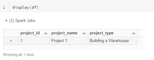
As with writing data, reading is a simple operation that requires one line of Python to read a dataset from Delta Lake. Once completed allows you to filter and transform data with a high degree of complexity. After the Data is loaded, you can display() command in Databricks to view the first 1000 rows (Figure 1).
new_df = spark.table(“demo_db.mock_projects_demo”)
Figure 1. Reading and displaying data from the Delta Lake format.
Inserting/updating Data
A common operation for databases and data warehouses is the inclusion of new / updated data, either through an append or upsert mechanism, which can be difficult for data lakes due to the lack of structure. However, these are standard operations using the DeltaLake format and, as such, performed with little code! The first example shows a simple append operation, while the second a more useful update mechanism based on a matching key (Figure 2).
Note an update can be done all in Spark as well, but you would have to read and write the entire table, which would be costly on a large dataset, whereas Delta Lake only updates the rows you request in the file.
df.write.format(“delta”).mode(“append”).saveAsTable(“demo_db.mock_projects_demo”)
deltaTable.update(
“project_type = ‘Building a Warehouse'”,
{“project_type”: “‘Building a Lake'”}
)
Here is what the table looks like before the update() method above is run:
And after:

Figure 2. Updating data stored in the Delta Lake format.
Deleting Data
The final basic operation worth discussing is deleting data, equivalent to removing a row of data in Excel or a SQL DELETE operation. As with the majority of these basic commands, it’s a one-line statement; Here, we are deleting all rows where project_name equals “project 1”:
deltaTable.delete(“project_name = ‘project 1′”)
It’s important to note that this doesn’t actually delete the physical Data on its own – you can still retrieve the data by looking at a version of data before the deletion, which helpful in undoing costly mistakes. You can, however, physically remove the data using a Vacuum command.
Basics Summary
Hopefully, based on this quick run-through, you’ve come to the same conclusion after implementing Lakehouse for clients: it is straightforward and easy to use. But you might be thinking, “This is all very well showing me a simple example; I want to see a more complex, more realistic example,” which is why we prepared such an example below.
Real-World Example: Updating a Slowly Changing Type 2 Dimension in Delta Lake
Background
For a more real-world example, we’ll be looking at a construction company that relies heavily on tabular data to store project milestones and finances, a feature common to many organisations. In our Data Lakehouse, we want a table for all our planned, live, and completed projects, such as the mock table below, which includes the associated name and type (Figure 3).
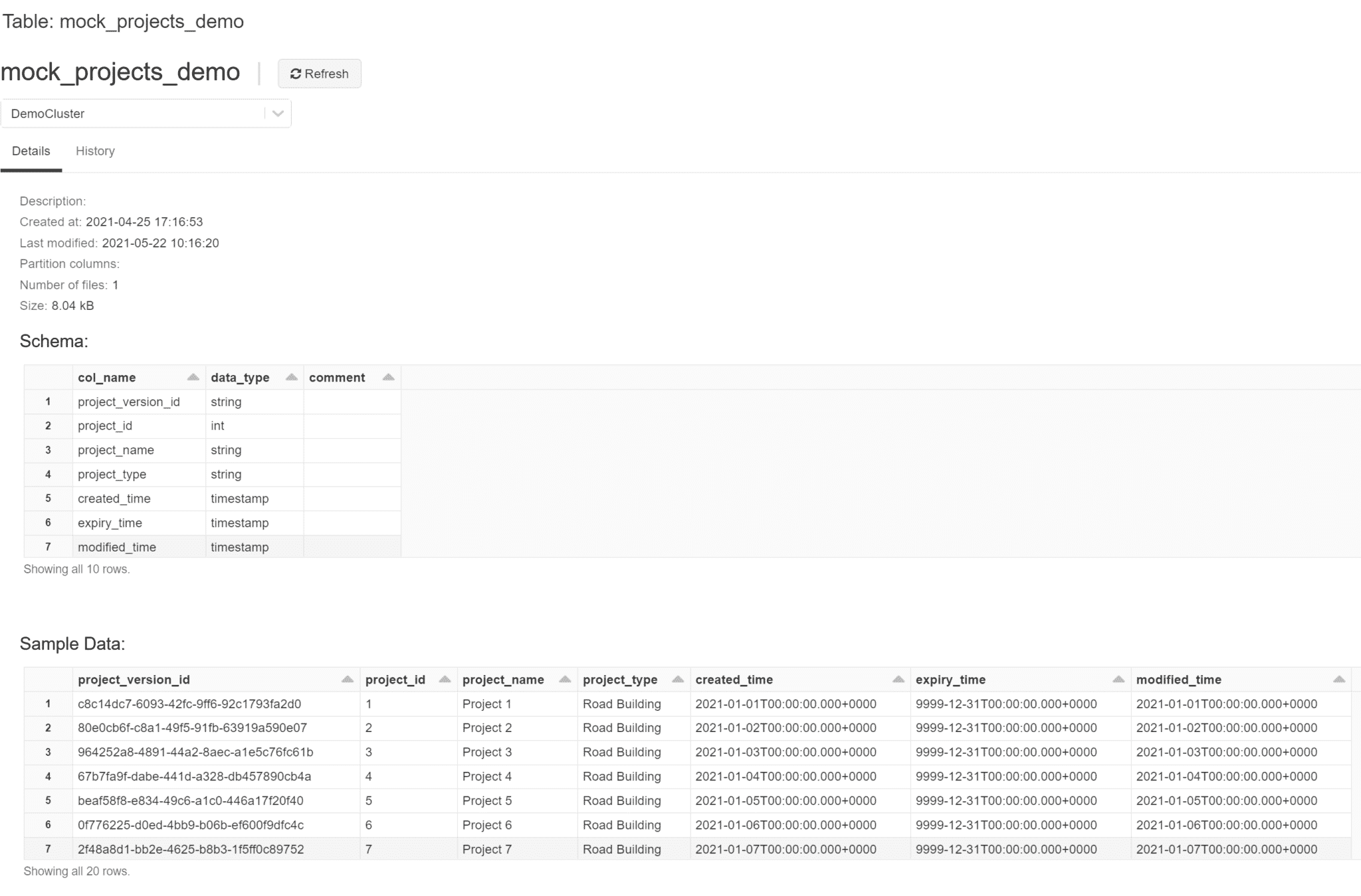 Figure 3. Databricks UI representation of a project dimension table.
This is what we call a Slow Changing Dimension (SCD) table of the type 2 variety. It is a very common table type in a Data Warehouse, especially if you are modelling your Data on a Star Schema. This dimension table would join to a “facts” table via its project_version_id, along with other dimensions like project date table or project worksite location table. Joining data into a wide format like this is common for auditing purposes or for machine learning applications, but it is cheaper to store in smaller, separated tables.
Using the above data, we can now show the process for updating said dimension table with a new set of data, as seen in Figure 4, which could be coming from anywhere: an application to update project dimensions, external database, data stream, or just a file; All of which can be easily handled by Spark, the processing engine that underpins the Lakehouse.
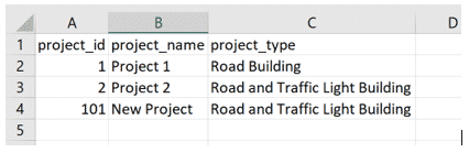
Figure 4. Updated project dimension table.
The new incoming data above covers the three most common actions that can happen when updating a dimension table with new data:
- The first row covers the scenario where new data matches existing data, so, therefore, it will be ignored.
- The second row covers the scenario where the project id matches attributes of the project that has changed (in this example, project_type), so we need to update this. This and the bullet point above is equivalent to updating a row in Excel, or a SQL UPDATE operation with a WHERE clause or MERGE operation.
- The third row covers the scenario where a new project has been created, so it simply needs appending to the existing data. This is equivalent to adding a new row in Excel or a SQL MERGE (an INSERT operation with an WHERE clause) operation.
Implementation
Now we can go through the process for updating our dimension, for which the code is shown in example 2 in the code appendix:
- Import stored functions to simplify the transformations and the required tables for the original and updated data.
- Find rows where project ID matches but project attributes do not. Here the new dataset (incoming_df) is being joined to an existing dataset on the project_id, and then we compare attributes, leaving behind rows where attributes do not match. Then we keep the new attributes and the original creation_time. Finally, we add columns that do not exist in the new data. Note how this contains only the row where project id from incoming Data matches the existing data, but the attributes are different (Figure 5).
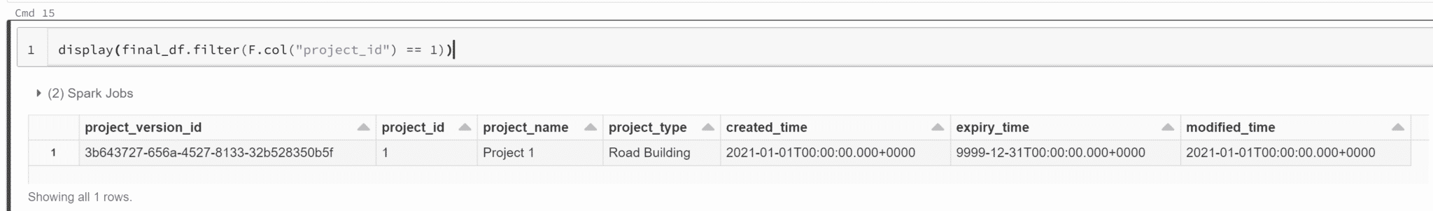
Figure 5. Updated dataframe with new attributes based on matching IDs
- Update rows in the old table with rows from step 2. This process updates the expiry time to the current date and time to show it is no longer the current version and then add in the row that is the new version of a project ID that we created in step 2.
- Add new rows. Here we are adding rows where the project id does not match, creating new projects in the table.
Results
No new rows have been added for project 1, as the attributes did not change (Figure 6).
Figure 6. Data for project 1, which matches the original dimension table.

A new row for project 2, as the project attributes have been updated in steps 2 and 3 (Figure 7). Additionally, if we just wanted to get the latest project characteristics, we would pass in an additional filter of getting all rows where expiry_time is higher than the current time and date (Figure 8).

Figure 7. Updated project dimension where new information is available for a project.

Figure 8. Finding the latest project attributes, where changes have occurred throughout the project
And finally, a new row for project 101 that we added in step 4 (Figure 9).

Figure 9. Addition of a new project and its attributes
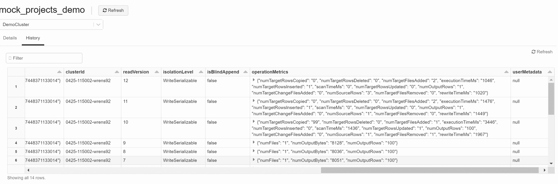
Also, as a bonus, Figure 10 shows the Delta Lake History page, detailing the changes to the underlying data after a few update operations. This page makes it possible to see the various versions of the data, allowing the user to more easily pick a version to roll back to before any unwanted changes were made. It also keeps track internally of the number of updated/inserted rows and their performance.
 Figure 10. Example of a Delta Lake history page detailing the changes to said dataset
Summary
Based on the above, Databricks Lakehouse can clearly handle common patterns of a Data Warehouse while still being a Data Lake, thus offering a substantial cost saving for many consumers. The above can be easily extended for more complex patterns, such as merging two or more datasets into one dimension. If you have any questions or queries on this post or anything related to Data, feel free to contact us.
Jake Watson is a Senior Data Engineer at Oakland, where he designs and builds scalable ETL process and data warehousing for clients.
Code appendix
Note the code was written in a Databricks notebook in Azure Databricks, though it should also work on the AWS and GCP versions of Databricks or in a custom Spark and Delta Lake environment. All the code is written in pySpark, which is the Python API of Apache Spark: there is also an API available for SQL, Java, and Scala.
Example 1: Pre determining a schema
schema = Type.StructType([T.StructField(“project_id”, T.IntegerType()),
Type.StructField(“project_name”, T.StringType()),
Type.StructField(“project_type”, T.StringType())])
df = spark.createDataFrame(incoming_list, schema=schema)
df.write.format(“delta”).mode(“overwrite”).saveAsTable(“demo_db.mock_projects_demo”)
Example 2: updating a slowly changing dimension table
- Import functions and tables:
from uuid import uuid4
import pyspark.sql.functions as F
import pyspark.sql.types as T
from delta.tables import *
# Build New Incoming Data.
incoming_list = [
[1, “Project 1”, “Road Building”],
[2, “Project 2”, “Road and Traffic Light Building”],
[101, “New Project”, “Road and Traffic Light Building”]
]
schema = T.StructType([T.StructField(“project_id”, T.IntegerType()),
T.StructField(“project_name”, T.StringType()),
T.StructField(“project_type”, T.StringType())])
incoming_df = spark.createDataFrame(incoming_list, schema=schema)
# Get Existing Data
existing_delta_lake = DeltaTable.forPath(spark, “<path to existing file>”)
- Find rows where project ID match but project attributes do not:
updated_df = (
incoming_df .alias(“updates”)
.join(existing_dl.toDF().alias(“projects”), “project_id”)
.where(“updates.project_type <> projects.project_type
OR updates.project_name <> projects.project_name”)
.select(“updates.project_id”, “updates.project_name”,
“updates.project_type”, “projects.created_time”)
.withColumn(“project_version_id”, uuid_udf())
.withColumn(“modified_time”, F.current_timestamp())
.withColumn(“expiry_time”,
F.to_timestamp(
F.lit(“30/12/9999 00:00”), “dd/MM/yyyy HH:mm”)
)
)
- Update rows in old table with rows from step 2
# Update old version of projects where ids match but the attributes do not.
existing_delta_lake.alias(“projects”).merge(
updated_df.alias(“updates”),
“projects.project_id = updates.project_id”)
.whenMatchedUpdate(
condition = “updates.project_type <> projects.project_type OR updates.project_name <> projects.project_name”,
set = {
“expiry_time”: F.current_timestamp()
}
).execute()
# Add new version of where ids match but the attributes do not.
(
existing_delta_lake.alias(“projects”).merge(
updated_df.alias(“updates”),
“projects.project_version_id = updates.project_version_id”
).whenNotMatchedInsertAll().execute()
)
- Add new rows
(
existing_delta_lake.alias(“projects”).merge(
incoming_df.alias(“new”), “projects.project_id = new.project_id”)
.whenNotMatchedInsert(
values = {
“project_version_id”: F.lit(str(uuid4())),
“project_id”: “new.project_id”,
“project_name”: “new.project_name”,
“project_type”: “new.project_type”,
“modified_time”: F.current_timestamp(),
“created_time”: F.current_timestamp(),
“expiry_time”: F.to_timestamp(F.lit(“30/12/9999 00:00”),
“dd/MM/yyyy HH:mm”),
}
)
.execute()
)